Visualizing gzip compression with Python!
Stephen Brennan • 22 September 2020Not that long ago, I found myself wanting to understand gzip. I didn’t necessarily want to learn to implement the algorithm, but rather I just wanted to understand how it was performing on a particular file. Even more specifically, I wanted to understand which parts of a file compressed well, and which ones did not.
There may be readily available tools for visualizing this, but I didn’t find anything. Since I know gzip is implemented in the Python standard libraries, and I’m familiar with Python plotting libraries, I thought I would try to make my own visualization. This blog post (which is in fact just a Jupyter notebook) is the result.
What to measure
Sometimes the hardest part of a data analysis problem is just figuring out what you want to measure. The data is all there, and you have a computer at your disposal, so the possibilities are endless. Knowing what to compute is tricky. In my case, I want to understand which parts of a file compress well. So it makes sense that whatever I visualize should include the position in the file along the X axis, and the compressed size along the Y axis. An uncompressed file would simply be a diagonal line. The better the compression, the more this line would stay under the diagonal line of an uncompressed file.
How to measure it?
Since Python supports gzip in the standard library, let’s see how we can measure these X and Y coordinates. First, let’s create a file with some compressed data. My favorite to use in this instance is Alice’s Adventures in Wonderland, downloaded from Project Gutenberg. We’ll compress it on the command line for simplicity.
(Note that code prefixed by ‘!’ is executed via bash - everything else is executed in Python).
!gzip -k alice.txt
!ls -lh alice*
-rw-r--r-- 1 stephen stephen 171K Sep 22 20:25 alice.txt
-rw-r--r-- 1 stephen stephen  60K Sep 22 20:25 alice.txt.gz
gzip does a pretty decent job at compressing this, far better than I could do myself. Now, let’s use Python to decompress just a little bit of it, and how much of the original file is consumed as we go.
import gzip
compressed = open('alice.txt.gz', 'rb')
gzip_file = gzip.GzipFile(fileobj=compressed)
In the above code, we save the open file object as compressed before giving it over to the GzipFile. That way, as we read the decompressed data out of gzip_file, we’ll be able to use the tell() method to see how far we are through the compressed file.
first_100_bytes = gzip_file.read(100)
first_100_bytes
b'\xef\xbb\xbfThe Project Gutenberg EBook of Alice\xe2\x80\x99s Adventures in Wonderland, by Lewis Carroll\r\n\r\nThis eBook'
compressed.tell()
8212
This feels disappointing. We only read 100 bytes and yet it took 8212 bytes of gzip to give us that data? Well, we have to consider that compression algorithms need to store some tables of data which help decompress the rest of the file, so we should cut gzip some slack. Let’s do this a few more times.
gzip_file.read(100)
b' is for the use of anyone anywhere at no cost and with\r\nalmost no restrictions whatsoever. You may '
compressed.tell()
8212
This feels wrong. After reading 8212 bytes of compressed data for the first 100 bytes, it takes zero bytes to get the next 100?
gzip_file.read(100)
b'copy it, give it away or\r\nre-use it under the terms of the Project Gutenberg License included\r\nwith '
compressed.tell()
8212
Clearly there is some buffering going on here. 8212 is suspiciously close to 8192 (20 bytes away) which is a power of two, and thus likely to be a common buffer size. Python’s file I/O machinery is responsible for the buffering, but we can actually get rid of it by disabling buffering.
gzip_file.close()
compressed.close()
compressed = open('alice.txt.gz', 'rb', buffering=0)
gzip_file = gzip.GzipFile(fileobj=compressed)
gzip_file.read(100)
compressed.tell()
8212
Hm. We made compressed an unbuffered file, but maybe GzipFile has its own internal buffering. To avoid this, let’s do a bad thing. We can actually set the buffer size for all I/O operations by modifying io.DEFAULT_BUFFER_SIZE. If we set it to a small value, then we can reduce the impact of buffering on our measurements. Just for fun, let’s try setting it to 1.
import io
old_buffer_size = io.DEFAULT_BUFFER_SIZE
io.DEFAULT_BUFFER_SIZE = 1
gzip_file.close()
compressed.close()

compressed = open('alice.txt.gz', 'rb', buffering=0)
gzip_file = gzip.GzipFile(fileobj=compressed)
gzip_file.read(100)
compressed.tell()
205
This seems much more believable. To read 100 bytes of decompressed data, gzip had to read 205 bytes of compressed data (again, this is probably due to tables and other header information). Let’s continue for a bit:
bytes_unc = 100
for _ in range(5):
    gzip_file.read(100)
    bytes_unc += 100
    bytes_cmp = compressed.tell()
    print(f'uncompressed: {bytes_unc} / compressed: {bytes_cmp}')
uncompressed: 200 / compressed: 279
uncompressed: 300 / compressed: 335
uncompressed: 400 / compressed: 376
uncompressed: 500 / compressed: 449
uncompressed: 600 / compressed: 541
We can see that after reading 400 uncompressed bytes, the gzip compression has caught up! 376 compressed bytes needed to be read to give us those 400. The gap continues to widen as we go on.
Now that we’re confident that this approach is giving us interesting data, let’s make some functions to get all of this data for a particular file, so we can visualize it!
gzip_file.close()
compressed.close()
io.DEFAULT_BUFFER_SIZE = old_buffer_size
That was just some cleanup. Since modifying the buffer size would likely impact other code we run, it’s best to only modify the buffer size when we need it, and reset it back to its original value when we’re done. This can be done with a context manager.
import contextlib
@contextlib.contextmanager
def buffer_size(newsize=1):
    old_buffer_size = io.DEFAULT_BUFFER_SIZE
    io.DEFAULT_BUFFER_SIZE = newsize
    try:
        yield
    finally:
        io.DEFAULT_BUFFER_SIZE = old_buffer_size


with buffer_size():
    print(f'size: {io.DEFAULT_BUFFER_SIZE}')
print(f'size: {io.DEFAULT_BUFFER_SIZE}')
size: 1
size: 8192
Now for a function to retrieve compressed and uncompressed sizes. We can do this with a “chunk size” as a parameter. The larger our chunk size, the fewer data points we will have, but the code will run faster. We used 100 as a chunk size above, which seems good enough, but I do prefer a good round number, so I’ll change it to 64.
import pandas as pd

def create_compression_curve(filename, chunksize=64):
    with buffer_size(1), open(filename, 'rb') as fileobj:
        gf = gzip.GzipFile(fileobj=fileobj)
        records = []
        read = 0
        while True:
            data = gf.read(chunksize)
            if len(data) == 0:
                break  # end of file
            else:
                read += len(data)
                records.append((read, fileobj.tell()))

    df = pd.DataFrame(records, columns=['uncompressed', filename])
    return df.set_index('uncompressed')


ccurve = create_compression_curve('alice.txt.gz')
ccurve
| alice.txt.gz | |
|---|---|
| uncompressed | |
| 64 | 176 |
| 128 | 224 |
| 192 | 271 |
| 256 | 315 |
| 320 | 345 |
| ... | ... |
| 174272 | 61351 |
| 174336 | 61362 |
| 174400 | 61379 |
| 174464 | 61404 |
| 174484 | 61417 |
2727 rows × 1 columns
The above function simply reads the gzipped file in chunks, measuring the distance we’ve gone through the compressed file each time, and adding it to a list of “records”. This list is converted into a Pandas Dataframe, which is commonly used to hold tabular data like this. We set the “uncompressed” column to be the “index”, since that’s what we’d consider the X-axis.
The result looks exciting! We can even go right ahead and plot it from here.
# Some style changes to make the plots more pretty
import matplotlib.pyplot as plt
import matplotlib as mpl
plt.style.use('ggplot')
mpl.rcParams['figure.figsize'] = [16, 8]

ccurve.plot()
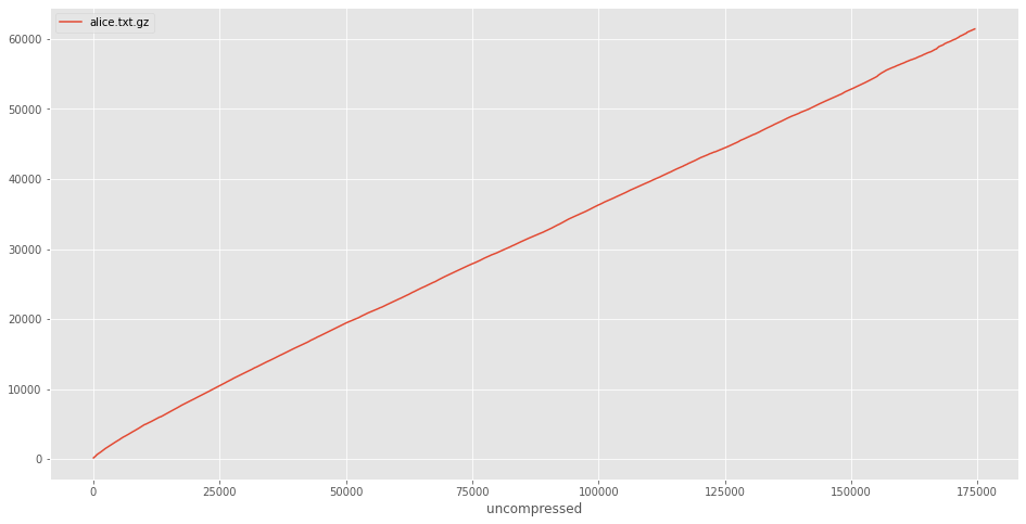
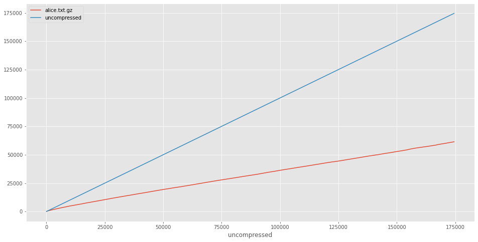
Well, I gotta give it to gzip – it’s pretty consistent. I can’t really see anything interesting in the plot, except that the gzipped data is smaller than the uncompressed version (duh). We can add this in to make it more explicit:
ccurve['uncompressed'] = ccurve.index
ccurve.plot()
What to do with this new power?
So, the result here seems to be blindingly mundane. gzip compresses reasonably well, it’s obviously better than uncompressed.
Well, let’s try to make things less mundane. First, a peek at the gzip(1) manual page indicates that it has different compression levels 1-9. I’ll let the manual do the explaining:
   -# --fast --best
          Regulate the speed of compression using the specified digit #, where -1
          or  --fast  indicates the fastest compression method (less compression)
          and -9 or --best indicates the slowest compression  method  (best  com‐
          pression).   The  default  compression level is -6 (that is, biased to‐
          wards high compression at expense of speed).
What if we used this compression curve plot to compare the gzip compression levels?
import os
files = []
for level in range(1, 10):
    os.system(f'gzip -k -S .gz.{level} -{level} alice.txt')
    files.append(f'alice.txt.gz.{level}')
    print(f'Created {files[-1]}')
Created alice.txt.gz.1
Created alice.txt.gz.2
Created alice.txt.gz.3
Created alice.txt.gz.4
Created alice.txt.gz.5
Created alice.txt.gz.6
Created alice.txt.gz.7
Created alice.txt.gz.8
Created alice.txt.gz.9
Above I went ahead and created all the different compression levels. Now, we can get compression curves for all of them and plot them:
ccurves = pd.concat([
    create_compression_curve(fn) for fn in files
], axis=1)
ccurves.plot(title="gzip Compression Level Comparison (Alice's Adventures in Wonderland)")
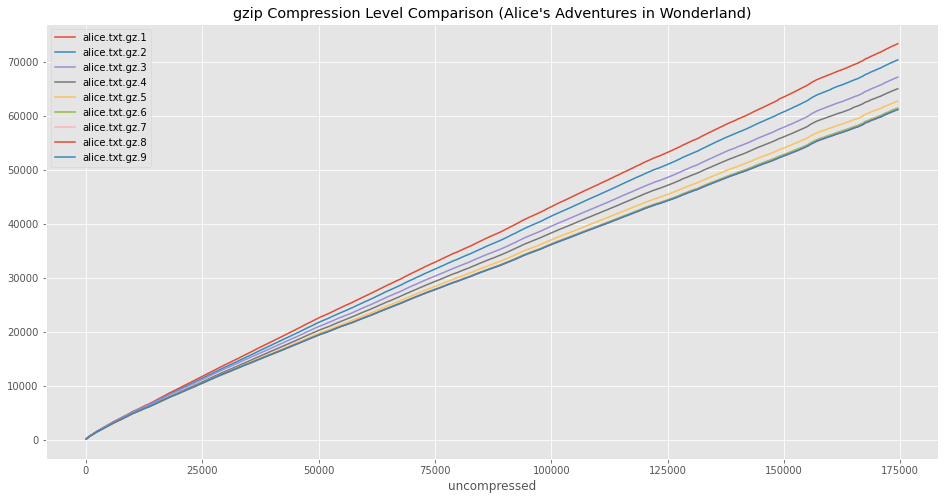
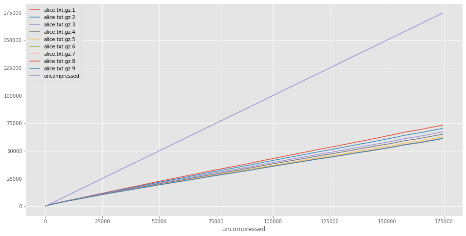
That seems slightly more interesting. The default compression level of 6 seems to be chosen well. Beyond level 6, the reduction in file size seems pretty difficult to notice. However, the difference between the compression ratios is rather small compared to the uncompressed line:
ccurves['uncompressed'] = ccurves.index
ccurves.plot()
Making an interesting graph
Ok, so we just saw that gzip’s compression levels do in fact work as the manual page describes. But at the end of the day everything just looks like a line. And this isn’t really that surprising. Human language is a textbook example of data which is easy to compress, and it’s pretty consistent. What if we created a file which wasn’t like that?
We could combine random data (difficult to compress) with human language to create regions of a file which compress at different ratios, and see what we get!
Below I’ll create a file using a series of dd commands, compress it, and plot it.
!dd if=alice.txt    of=special.data bs=4096 count=10
!dd if=/dev/urandom of=special.data bs=4096 count=10 oflag=append conv=notrunc
!dd if=alice.txt    of=special.data bs=4096 count=10 oflag=append conv=notrunc skip=10
!dd if=/dev/urandom of=special.data bs=4096 count=10 oflag=append conv=notrunc
!dd if=alice.txt    of=special.data bs=4096 count=10 oflag=append conv=notrunc skip=20
!dd if=/dev/urandom of=special.data bs=4096 count=10 oflag=append conv=notrunc
!dd if=alice.txt    of=special.data bs=4096 count=10 oflag=append conv=notrunc skip=30
!dd if=/dev/urandom of=special.data bs=4096 count=10 oflag=append conv=notrunc
!gzip -k special.data
10+0 records in
10+0 records out
40960 bytes (41 kB, 40 KiB) copied, 0.000172505 s, 237 MB/s
10+0 records in
10+0 records out
40960 bytes (41 kB, 40 KiB) copied, 0.000732935 s, 55.9 MB/s
10+0 records in
10+0 records out
40960 bytes (41 kB, 40 KiB) copied, 0.000242876 s, 169 MB/s
10+0 records in
10+0 records out
40960 bytes (41 kB, 40 KiB) copied, 0.000810064 s, 50.6 MB/s
10+0 records in
10+0 records out
40960 bytes (41 kB, 40 KiB) copied, 0.000156087 s, 262 MB/s
10+0 records in
10+0 records out
40960 bytes (41 kB, 40 KiB) copied, 0.000727009 s, 56.3 MB/s
10+0 records in
10+0 records out
40960 bytes (41 kB, 40 KiB) copied, 0.000379906 s, 108 MB/s
10+0 records in
10+0 records out
40960 bytes (41 kB, 40 KiB) copied, 0.00074872 s, 54.7 MB/s
special_ccurve = create_compression_curve('special.data.gz')
special_ccurve.plot(title='Compression curve: alternating random data and text')
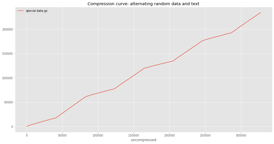
Here’s some fun data! I know the above plot looks like it only has a few data points, but it actually has one point every 64 bytes along the X axis. The piecewise nature of the plot is just due to how obviously different gzip performs on the two different types of data. The first segment is text data, and so the slope is not very steep. The second segment is random data, which does not compress well, and so the slope is steep. This alternates for all the segments.
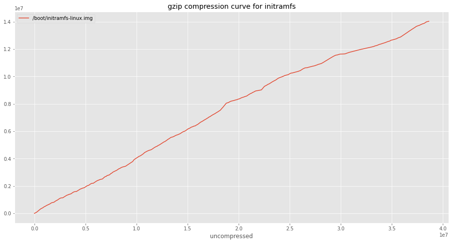
What’s in your initramfs?
An initramfs is a small filesystem which gets loaded just after your OS boots. It contains drivers and configuration data necessary to get your computer to the point where it can mount the real filesystem in all its glory. It also happens to be (on my machine) gzip compressed.
ccurve_initramfs = create_compression_curve('/boot/initramfs-linux.img')
ccurve_initramfs.plot(title='gzip compression curve for initramfs')
What’s next?
Who knows. I didn’t really have a purpose in doing this, beyond curiosity. And as you can see, not much came from it beyond some plots of squigly lines.
There are some other compression algorithms implemented in the Python standard library. I could try to compare compression algorithms on the same file, which could be interesting.
I could also try to find more exciting compressed files. There must be something out there which creates a cool compression curve!
In any case, I’d encourage you, the reader, to hack on this code and find something interesting for yourself.

Stephen Brennan's Blog is licensed under a Creative Commons Attribution-ShareAlike 4.0 International License