Fare Hacking on BART
Stephen Brennan • 23 July 2016Imagine that you’re taking a long train ride on the BART. Maybe from Millbrae to North Concord. Chances are, at the very same moment, somebody else is going the other direction. For example, maybe from Pittsburgh/Bay Point to San Bruno. In case you haven’t memorized BART’s stops, here’s a useful map illustrating these rides:
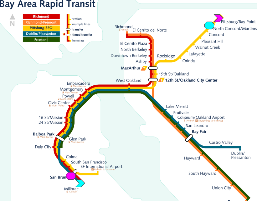
You’re the cyan rider (starting at the chevron and ending at the octagon), and the other person is in magenta.
Now, if you both bought correct tickets, your trips would cost a little more than $7 each. That’s not unreasonable, but there’s a way you could pay less, so long as you know the Magenta rider.
- Instead of buying a ticket for Millbrae to North Concord, you just buy a ticket for Millbrae to San Bruno.
- Magenta buys a ticket for Pittsburgh/Bay Point to North Concord.
- Halfway through, you both get off your trains, meet on the platform, and swap your tickets.
- Then you continue on the next train to your destinations.
This ends up saving both of you around $5, but in the process you lose 20 minutes standing around on a platform in Oakland! Probably not worth it. But, what if there were a way to do this electronically so that you never had to get off the train? After all, Clipper Cards (the electronic ticket of choice on the BART system) use NFC, which is a technology built into some smartphones. Although Clipper Cards currently aren’t cloneable or spoofable, if they were, an app could theoretically use the principle from above to swap tickets around, reducing everyone’s fares!
I’ve had this idea bouncing around in my head for a couple weeks. Thursday and Friday were Hackathon days at Yelp, which gave me the perfect opportunity to take a shot at making this app. I successfully implemented what I think is a pretty neat algorithm and API, and then ran it on some real BART data. My results indicate that an app like this could save its users between 20 and 40% on BART fares, depending on time of day. Read on for all the gory details—I think it’s pretty fascinating!
One final note before I dive in: this algorithm is essentially large scale ticket swapping, which is obviously illegal and unethical. I don’t believe that it would be ethical to use this in the real world. I value safe and smooth travel more than I value the 20-40% of my fare I could save by stealing from BART. With that said, I still think this is a really cool problem, and since Clipper cards are not cloneable, this work can’t be used to facilitate this large-scale theft.
The algorithm
In order to write an algorithm, we should always step back and formulate the problem as clearly as we can. In this case, the input to our problem is a bunch of people who would like to go from point A to point B. Our job is to “purchase” tickets that we can assign to people on entry, and then swap to other people on exit, so that we minimize the total cost of these tickets.
Let’s go back to the toy example I presented in the beginning. Why does it work? What is the fundamental property we are taking advantage of? It’s actually pretty simple: BART would like to enforce that everyone who travels from point A to point B buys a ticket for that source and destination. However, with just turnstiles at stations, they can’t enforce that. The best they can enforce is that each person entering a station has a valid ticket for a trip starting there, and that each person exiting a station has a valid ticket for a trip ending there.
This gives us a set of constraints. Our algorithm can purchase whatever tickets it wants, so long as we end up with the same number of people entering and leaving each station. Since we’re minimizing the total cost of the tickets, we have a classic optimization problem. In particular, this problem can be expressed as an Integer Linear Program.
Linear programs are math problems where you are trying to choose
values for a vector (i.e. a list) of variables  , such that you minimize a
cost function. Typically, each variable
, such that you minimize a
cost function. Typically, each variable  in has an associated cost
 , and so the cost function is just the sum of the ’s times their
costs. But, you have to satisfy some constraints, which are usually expressed as
equations, like this:
, and so the cost function is just the sum of the ’s times their
costs. But, you have to satisfy some constraints, which are usually expressed as
equations, like this:

We can have lots of constraints we need to satisfy, so we typically number the
constraints from one to  . We can compactly write all the constraints using
a matrix form like this:
. We can compactly write all the constraints using
a matrix form like this:

Here,  is an row (one for each constraint) by
  column (one for
each variable) matrix containing the coefficients
column (one for
each variable) matrix containing the coefficients  from all the
constraints. Usually we also have the constraint that
from all the
constraints. Usually we also have the constraint that  , and for
integer linear programs, we also need to make sure that our solutions for
are integers. Since linear programs are pretty common problems to solve, there
are plenty of existing solvers that can solve them reasonably quickly. If you
can write a problem as a linear program and come up with ,
, and for
integer linear programs, we also need to make sure that our solutions for
are integers. Since linear programs are pretty common problems to solve, there
are plenty of existing solvers that can solve them reasonably quickly. If you
can write a problem as a linear program and come up with ,  , and the
costs
, and the
costs  , you can use these linear programming libraries to solve your
problem for you. So let’s formulate this as an integer linear program!
, you can use these linear programming libraries to solve your
problem for you. So let’s formulate this as an integer linear program!
In this particular problem, we have a variable for every single pair of
stations you could start at and end at. will represent how many tickets we
buy for that start/end pair. There are 45 BART stations, which means that we
have 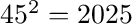 different variables. The cost for each variable is provided
in a fare schedule, available from BART’s website. The one value
that is missing from this schedule is the cost of a trip that starts and ends at
the same station. You’d think that this would be free, but people would take
advantage of that. So BART charges $5.75 for this and markets it as a chance to
“explore”1 their train system!
different variables. The cost for each variable is provided
in a fare schedule, available from BART’s website. The one value
that is missing from this schedule is the cost of a trip that starts and ends at
the same station. You’d think that this would be free, but people would take
advantage of that. So BART charges $5.75 for this and markets it as a chance to
“explore”1 their train system!
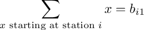
I already outlined the constraints in words, and now we can actually express them mathematically. The first constraint was that the number of tickets starting at any station has to be equal to the number of travelers starting at that station. So, the constraint is:
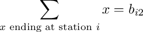
We have one of these constraints for each station. We’ll call them the source constraints. The second type of constraint was that the number of tickets ending at any station has to be equal to the number of travelers who want to go to that station:
And these are our destination constraints. Together, the source and
destination constraints can be represented in using the matrix form  .
The matrix is pretty large, with 90 rows and 2025 columns! Regardless of how big
it is, this should mean that we’re done. We can use a linear programming library
to solve the problem.
.
The matrix is pretty large, with 90 rows and 2025 columns! Regardless of how big
it is, this should mean that we’re done. We can use a linear programming library
to solve the problem.
Integer linear programs are hard
Actually, we may not yet be done. You see, while linear programs are solvable on average in a reasonable (a.k.a. polynomial) amount of time, integer linear programs are not. They are NP-hard, which means that you can’t expect to find a solution in a reasonable amount of time.
However, sometimes a particular instance of an integer linear program is not that hard. For some problems, if you just “forget” the constraint that your solutions should be integers, and solve the problem as a normal linear program, you’ll always get integer solutions anyway.
This happens whenever your constraint matrix is totally unimodular. I
won’t explain what that is, but it turns out that our matrix is
unimodular!2 So this means that we can just use a linear
programming library to solve it. In fact, here is the code I used to do it:
b = np.hstack([src_sum(self.traveler_matrix),
               dst_sum(self.traveler_matrix)]).astype(np.float)

A_src_const = np.repeat(np.identity(self.num_stations),
                        self.num_stations, axis=1)
A_dst_const = np.hstack(
    [np.identity(self.num_stations) for _ in range(self.num_stations)])
A = np.vstack([A_src_const, A_dst_const])

c = self.fare_matrix.reshape(self.num_stations ** 2)

self.res = scipy.optimize.linprog(c, A_eq=A, b_eq=b)
There is some stuff missing—you can see the code in its original context here. The point of this sample is to demonstrate that formulating your problem as a linear program can make for a very nice, compact, and clean solution! However, the limitation is that your solution is only as good as the underlying linear programming library!
Regular linear programming is hard too
It turns out that not every linear programming library is created equal.
Sometimes, they don’t work right. Since my project was in Python, I used NumPy
and SciPy, the industry and academic standard toolchain for math in Python.
SciPy’s implementation of the simplex algorithm, like most implementations,
has two phases. In the first, it searches for any solution that can satisfy the
constraints (this is called a basic feasible solution). In the second, it takes
this solution and modifies it until it finds the optimal solution. However,
occasionally SciPy wasn’t able to find a basic feasible solution in the first
step, even though in this case there is always a very simple one: just buy a
ticket for each person’s ride directly. It’s not optimal, but it satisfies the
source and destination constraints. Unfortunately, I wasn’t really able to get
around this problem, so it was right back to square one for me.
Edit (December 2016): My solution using SciPy’s linear programming solver did not work, because I sometimes gave it linearly dependent constraints. I wasn’t aware that was the problem. You can read more about this issue and how I’ve resolved it here.
But this was a hackathon, and there’s no giving up at a hackathon! If one thing doesn’t work, you just find a new way to do it. And you don’t waste too much time going down rabbit holes trying to fix it. So instead I decided to come up with a custom algorithm from scratch for this problem.
The other algorithm
So even though this problem can be expressed as a linear program doesn’t mean that you have to solve it with one. In fact, simply knowing that a problem can be written as a linear program can give you a lot of insight into how you should write a custom algorithm for solving it. For instance, a problem that can be expressed as a linear program is convex, which is very convenient. This means that we can use a simple algorithm to solve it.
To understand why, think of a very simple “optimization” problem: finding the highest point in an area of land. If the area of land you’re on has a single hill, it’s probably convex, meaning that there are no valleys or other indented regions. This means you can follow the straightforward strategy of always following the steepest slope. No matter what, this approach is guaranteed to get you to the top of the hill.

Above: Windows XP’s desktop background, representing a convex optimization problem. There is only one peak. Source
On the other hand, if the area you’re on has multiple hills, it’s definitely not convex: there’s a valley in between! If you follow the same strategy as above, you might end up on top of the highest hill, but you also might end up on a different peak: a local optimum.

Above: An non-convex area with many “local” peaks. Source
These examples may seem silly or contrived, but in fact many optimization problems boil down to something as simple as “climbing a hill”, but instead of changing your X and Y coordinates, you can change many more variables: approximately 2025 in the case of the problem of BART fare minimization. But since this problem is convex, it’s rather simple: like finding the top of a single hill, but in 2025 dimensional space!
So how do we find our way up this 2025 dimensional hill? To answer that
question, let’s represent our problem a bit differently: with a matrix. We’ll
label both the rows and the columns with stations: the rows are the starting
stations, and the columns are ending stations. A number in row  ,
column
,
column  means that people are riding from station to station
. We’ll call this our traveler matrix,
means that people are riding from station to station
. We’ll call this our traveler matrix,  . Here’s a small example with
four stations:
. Here’s a small example with
four stations:
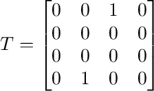
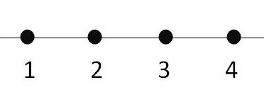
In this example, one traveler wants to go from station 1 to 3, and another wants to go from station 4 to 2. If you imagine the stations in a line, it’s a bit easier to visualize.
If you imagine that the fare is $1 for every “link” in this simple train route,
then the fare matrix  would look something like this:
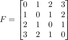
You could get the total fare for everyone in this little system by taking each element in the “traveler matrix” and multiplying it with its corresponding element in the “fare matrix”, then adding them all up3. For the example travelers, the total fare is $4.
According to our constraints, we are free to do anything we’d like to the traveler matrix (which we can refer to now as a ticket matrix, since it will represent the tickets our algorithm buys), so long as we maintain the source and destination constraints. In this matrix formulation of the problem, this simply means that we can’t do anything to the matrix that changes its row or column sums.
There’s a very convenient way to change a matrix so that you don’t modify the
row and column sums: simply find two entries in different rows and columns that
are greater than zero. They form two corners of a rectangle in the matrix.
Subtract however many tickets you want from both those entries, and add them to
the other two corners of the rectangle. Let’s do this with the previous example
:
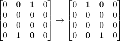
If we look back at the fare matrix, we can see that this transformation actually
lowered the total fare of the system from 4 to 2! This is because we went from
having tickets  and
and  , which both cost $2 to simply having
tickets
, which both cost $2 to simply having
tickets  and
and  , which both cost $1.
And in fact, that’s pretty much the whole algorithm! All my custom algorithm does is look in the matrix for pairs where it can perform this swap, and do it if it will lower the total fare. Since lowering the fare is the equivalent of going “uphill” in our 2025 dimensional problem, we know that as long as we keep going uphill, we’ll eventually reach the peak. Thank you, convexity!
This algorithm, as I implemented it, is not very smart or efficient, but it’s definitely “hackathon complete”. It does the job!
The implementation
After I got this algorithm settled, the next order of business was implementing
it in a realistic way: as if it were the basis of a real app that would be
deployed to real users. So I made a REST API, which clients (apps) can use. The
most important endpoint is /travel. Whenever a client sends a request to
/travel, it provides a source, destination, and a piece of identifying info,
like a name or a clipper card number. The server adds that traveler to the
current “batch” of travelers waiting to have their tickets swapped. The server
returns a unique ID to each traveler which they can look up later to get their
exit ticket. Then, at some point an admin requests the /calculate endpoint,
which instructs the server to perform the ticket swapping algorithm on the
current batch of travelers. The server calculates it all and returns the
original and optimal fare cost. After that, travelers can look up their ID on
the /result/<id> endpoint to get their exit ticket.
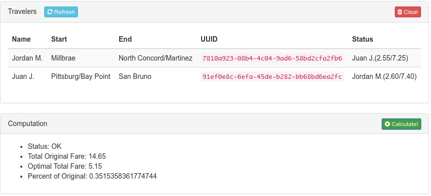
The only client I created was an “admin” website. It has two panels. The first is a manual entry form, which allows you to manually add travelers and then do the fare swapping algorithm. Here you can see it working on the example from the beginning of this article:
The second is a simulation interface. It allows you to upload a day’s worth of BART origin-destination data in CSV format (available here). It will then send this all to the server, running the algorithm once for each hour of data. Essentially it can simulate a whole day of real BART traffic going into the app! As the simulation progresses, the site graphs a few performance measures to see how well the algorithm reduces fares. The results are pretty fascinating!
The results
I did two different simulations: one on a typical weekday with rush hour commute patterns (Thursday, August 6, 2015) and one on a weekend (Saturday, August 8, 2015). Below is the “savings” graph my simulation produced on the weekday. It plots the amount of money riders would save each hour if they all were using my fare swapping algorithm.
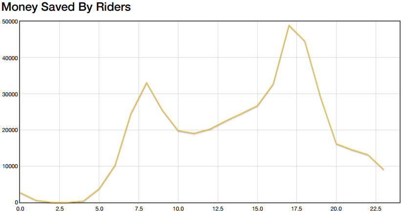
You can very clearly see two peaks during rush hour traffic. Even more exciting are the raw numbers: the graph peaks at $50,000 saved for a single hour during afternoon rush hour. During most operating hours the algorithm saves at least $20,000 per hour. Note that these savings assume that riders are paying the fare price listed on the fare schedule, passes are not taken into account here.
Perhaps more important than knowing the amount of money saved is knowing what fraction of their original fares riders would pay with the ticket swapping method:
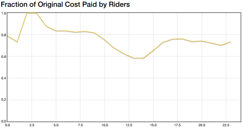
It appears that the savings fluctuate between 20% and 40%. If you look carefully, you’ll notice that the regions of the graph with 20% savings correspond to the rush hour traffic peaks from above. Savings are probably less during rush hour because most of the traffic is directed between work areas and residential areas. There are fewer swaps the algorithm can make in this situation.
This hypothesis is supported by looking at the same plot from the weekend simulation:
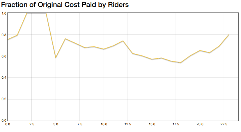
The savings are between 30% and 40% on this plot, likely because the traffic doesn’t have the directed flow that rush hour has.
Conclusion
Over the course of Thursday and Friday, I came up with an algorithm for swapping BART riders’ tickets to minimize their fares. I implemented it, wrapped it in a rough “API”, and evaluated its performance on real BART ridership data. The results? A hefty 20-40% discount on your train rides, and some neat visualizations of BART traffic patterns to boot.
Would it work in the real world? Maybe, if you assume that a mechanism for “cloning” Clipper Cards could become available some day. Disregarding that major barrier, there are still some problems that would have to be solved in a real world application of this algorithm:
- Adoption: The simulation results are so rosy because they assume everyone participates in the algorithm. Like social networks, the app might not be very good without a lot of users.
- Scheduling: My simulation ran the algorithm on a full hour of riders. In reality, you’d need to run it on smaller time increments (no larger than 10 minutes) so that riders wouldn’t be waiting on the app just to leave the station. I have plenty of interesting ideas for how to address this problem, but not enough hackathon time to try them.
- Performance: My algorithm is rather slow right now (a day’s simulation took around 40 minutes, although that does include some overhead from API requests). There are plenty of low hanging fruit for speeding it up, but I didn’t have time during the hackathon.
In any case, since I have no idea of launching a “stealing from BART” app any time soon, these “future work” problems will have to go unsolved.
This was a really enjoyable problem to solve. I learned a lot from it, and I got to apply some concepts that you normally just learn about in school. Hopefully people will enjoy reading about it as much as I enjoyed doing it!
If you want to learn more, check out the code on GitHub.
Edit (December 2016): An update to this post can be found here.
Footnotes
 . But I had to look that up on

Stephen Brennan's Blog is licensed under a Creative Commons Attribution-ShareAlike 4.0 International License